
Elasticsearch is the most popular open-source enterprise search engine widely used in the industry. We have learned what it is and why it is so fast. We have also learned how to use Elasticsearch in Python. An index laptops-demo have been created and filled with some sample data on which the queries in this article will be based. If you haven’t read these two articles yet, it’s recommended to read them first. However, if you already have some knowledge about Elasticsearch, you can go ahead with this article with no problem.
In this article, we will use the Console of the Dev tools in Kibana to build the queries in Elasticsearch Domain Specific Language (DSL). Kibana is a free and open frontend application that sits on top of the Elastic Stack, providing search and data visualization capabilities for data indexed in Elasticsearch. Kibana also acts as the user interface for monitoring and managing an Elastic Stack cluster. It is very convenient to write Elasticsearch queries in Kibana because there are hints and autocompletion for indices, fields, and commands. The queries built-in Kibana can be used directly in other languages like Python. Therefore, it is always a good idea to write and test Elasticsearch queries in Kibana and then implement them in other languages.
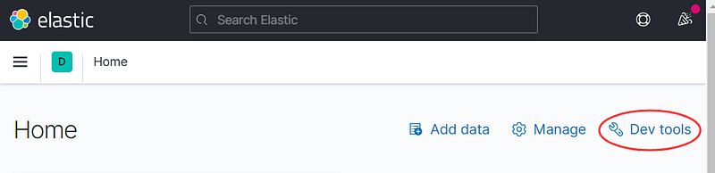
If you have installed Elasticsearch and Kibana on your computer or have started the corresponding Docker containers as in the previous article, you can open your browser and navigate to http://127.0.0.1:5601 to open the UI for Kibana. On the first page opened, click Explore on my own to work with our own data. If you don’t want to follow along, you can also learn by reading the queries and explanations in this article.

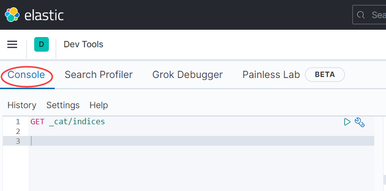
In the next page opened, click Dev Tools to open the Console:
Basic Elasticsearch queries for the Create, Read, Update and Delete (CRUD) operations for indices.
Create an index:
PUT /test-index
You can only run this command once, otherwise, you will see the error that the resource already exists. Note that the leading forward slash (/)is optional, you can omit it and the result will be the same.
Check the indices in the cluster:
GET _cat/indices
You can see the index just created, as well as some system indices created automatically.
Update the settings of an index:
PUT test-index/_settings
{
  "settings": {
    "number_of_replicas": 2
  }
}
You need to specify the _settings endpoint, otherwise you will see the same error of creating an index with an existing name.
Delete an index:
DELETE test-index
Basic Elasticsearch queries for the Create, Read, Update and Delete (CRUD) operations for documents.
In Elasticsearch, an index is like a table and a document is like a row of data. However, unlike the columnar data in relational databases such as MySQL, the data in Elasticsearch are JSON objects.
Create a document:
PUT test-index/_doc/1
{
  "name": "John Doe"
}
This query will create the index automatically if it doesn’t already exist. Besides, a new document with a name field is created.
Read a document:
GET test-index/_doc/1
Update a document by adding an age field.
POST test-index/_update/1
{
  "doc": {
    "age": 30
  }
}
Note that you must use the POST command to update a document. The fields to be updated are specified in the doc field.
Delete a document:
DELETE test-index/_doc/1
Now we have some feelings about the CRUD operations for Elasticsearch indices and documents. We can see that writing Elasticsearch queries is just like making RESTful API requests, using the GET, POST, PUT and DELETE methods. However, a major difference is that we can pass a JSON object to the GET method, which is not allowed in the regular REST GET method.
In the remaining part of this article, we will focus on how to search an Elasticsearch index with basic and advanced queries. To get started, we need to have some data in our index. If you haven’t followed the Elasticsearch and Python article and generated the laptops-demo index with Python, you need to create the index and populate it with some data as demonstrated below.
First, run the following command to create the index with predefined settings and mappings.
PUT laptops-demo
{
  "settings": {
    "index": {
      "number_of_replicas": 1
    },
    "analysis": {
      "filter": {
        "ngram_filter": {
          "type": "edge_ngram",
          "min_gram": 2,
          "max_gram": 15
        }
      },
      "analyzer": {
        "ngram_analyzer": {
          "type": "custom",
          "tokenizer": "standard",
          "filter": [
            "lowercase",
            "ngram_filter"
          ]
        }
      }
    }
  },
  "mappings": {
    "properties": {
      "id": {
        "type": "long"
      },
      "name": {
        "type": "text",
        "analyzer": "standard",
        "fields": {
          "keyword": {
            "type": "keyword"
          },
          "ngrams": {
            "type": "text",
            "analyzer": "ngram_analyzer"
          }
        }
      },
      "brand": {
        "type": "text",
        "fields": {
          "keyword": {
            "type": "keyword"
          }
        }
      },
      "price": {
        "type": "float"
      },
      "attributes": {
        "type": "nested",
        "properties": {
          "attribute_name": {
            "type": "text"
          },
          "attribute_value": {
            "type": "text"
          }
        }
      }
    }
  }
}
In this query, we create an index called laptops-demo. The settings section specifies that a filter called ngram_filter and an analyzer called ngram_analyzer is created. The mappings section specifies the schema for the documents to be created. Especially, the name field has multiple fields and the ngrams field is analyzed with ngram_analyzer created in the settings section. More details will be introduced for the settings and mappings later in this article.
As to the documents to be created, you can download this JSON file. The content of this JSON file has a format required by the bulk API:
{ "index" : { "_index" : "test", "_id" : "1" } }
{ "field1" : "value1" }
{ "create" : { "_index" : "test", "_id" : "2" } }
{ "field1" : "value3" }
{ "update" : {"_index" : "test", "_id" : "1" } }
{ "doc" : {"field2" : "value2"} }
{ "delete" : { "_index" : "test", "_id" : "2" } }
Key points:
- Both the
indexandcreateactions would create a new index and expect a source on the next line. The difference is thatcreatefails if a document with the same ID already exists in the target, whileindexadds or replaces a document as necessary. updateupdates an existing index and expects the fields to be updated on the next line.deletedeletes a document and does not expect a source on the next line.
Only the index action will be used in this example. We can use the curl command to call the bulk API and fill the index with the data in the JSON file.
curl -s -H "Content-Type: application/x-ndjson" -XPOST "http://localhost:9200/_bulk" --data-binary "@laptops_demo.json"
application/x-ndjson specifies that the data file is a Newline Delimited JSON where the line separator is the new line character \n and each line is a valid JSON value.
On Windows, if you can’t run curl properly, you may need to run this command in the terminal to use the right curl.
Remove-item alias:curl
Check these two posts about using curl on Windows:
If the curl command finishes successfully, and the documents would be added to the laptops-demo index. To check all the documents in an index, run this command:
GET laptops-demo/_search
It is the short version for:
GET laptops-demo/_search
{
  "query": {
    "match_all": {}
  }
}
You should be able to see all the documents added from the JSON file. Now that the index and documents are ready, we can start searching.
We already know how to check all the documents in the index. By default, all the fields are returned which can be difficult to read. To show only specific fields, we can specify the _sources keyword:
GET laptops-demo/_search
{
  "query": {
    "match_all": {}
  },
  "_source": ["name"]
}
If you don’t want to see the source at all, you can set _source to false:
GET laptops-demo/_search
{
  "query": {
    "match_all": {}
  },
  "_source": false
}
As the name implies match_all matches everything. To search based on some conditions, we can use the match keyword. For example, to search for all laptops whose name contains Apple:
GET laptops-demo/_search
{
  "query": {
    "match": {
      "name": "Apple"
    }
  }
}
We know from the mappings above that the name field is a text field and will be analyzed. In simple words, analyzing means to lower case the text string, split it into tokens, and remove punctuations. You can read more about analyzing at this link.
To see how a text will be analyzed, we can use the analyze endpoint:
GET laptops-demo/_analyze
{
  "text": "Apple MackBook!",
  "analyzer": "standard"
}
Here we use a standard analyzer, which as mentioned above, will lower case the text, split it into tokens and remove punctuations:
{
  "tokens" : [
    {
      "token" : "apple",
      "start_offset" : 0,
      "end_offset" : 5,
      "type" : "<ALPHANUM>",
      "position" : 0
    },
    {
      "token" : "mackbook",
      "start_offset" : 6,
      "end_offset" : 14,
      "type" : "<ALPHANUM>",
      "position" : 1
    }
  ]
}
Since we defined a special analyzer ngram_analyzer in the settings of the index, let’s use this analyzer to analyze our text and see what we will get:
GET laptops-demo/_analyze
{
  "text": "Apple MackBook!",
  "analyzer": "ngram_analyzer"
}
We can see a bunch of N-grams is generated:
{
  "tokens" : [
    {
      "token" : "ap",
      "start_offset" : 0,
      "end_offset" : 5,
      "type" : "<ALPHANUM>",
      "position" : 0
    },
    {
      "token" : "app",
      "start_offset" : 0,
      "end_offset" : 5,
      "type" : "<ALPHANUM>",
      "position" : 0
    },
    {
      "token" : "appl",
      "start_offset" : 0,
      "end_offset" : 5,
      "type" : "<ALPHANUM>",
      "position" : 0
    },
    {
      "token" : "apple",
      "start_offset" : 0,
      "end_offset" : 5,
      "type" : "<ALPHANUM>",
      "position" : 0
    },
    {
      "token" : "ma",
      "start_offset" : 6,
      "end_offset" : 14,
      "type" : "<ALPHANUM>",
      "position" : 1
    },
    {
      "token" : "mac",
      "start_offset" : 6,
      "end_offset" : 14,
      "type" : "<ALPHANUM>",
      "position" : 1
    },
    {
      "token" : "mack",
      "start_offset" : 6,
      "end_offset" : 14,
      "type" : "<ALPHANUM>",
      "position" : 1
    },
    {
      "token" : "mackb",
      "start_offset" : 6,
      "end_offset" : 14,
      "type" : "<ALPHANUM>",
      "position" : 1
    },
    {
      "token" : "mackbo",
      "start_offset" : 6,
      "end_offset" : 14,
      "type" : "<ALPHANUM>",
      "position" : 1
    },
    {
      "token" : "mackboo",
      "start_offset" : 6,
      "end_offset" : 14,
      "type" : "<ALPHANUM>",
      "position" : 1
    },
    {
      "token" : "mackbook",
      "start_offset" : 6,
      "end_offset" : 14,
      "type" : "<ALPHANUM>",
      "position" : 1
    }
  ]
}
These N-grams are useful for search-as-you-type or autocompletion, let’s try to search by a partial input:
GET laptops-demo/_search
{
  "query": {
    "match": {
      "name.ngrams": "Appl"
    }
  }
}
In this query, you can also get all the Apple laptops. If you search by Appl in the name field rather than name.ngrams field, you can’t find anything because the name field is analyzed by the standard analyzer and thus does not have the N-grams.
You might be wondering what’s the relationship between the name field and name.ngrams field. Well, this is called multi-fields which is to index the same field in different ways for different purposes. As a text field is always analyzed, we often add some additional fields for it. For example, a keyword type field is often added to a text field. The keyword type means the text will be treated as it is and won’t be analyzed. Multi-fields for the same field can be analyzed with a different analyzer. In this article, the name field is analyzed with the standard analyzer and the name.ngrams field is analyzed with a custom ngram_analyzer, which can be useful in different cases.
We have learned how to search a text field with the match query. There are also fields of other types such as long and float, these fields are like the keyword type of the text field and won’t be analyzed. If we don’t want the query input to be analyzed in searching, we can use the term query:
GET laptops-demo/_search
{
  "query": {
    "term": {
      "name.keyword": {
        "value": "Apple MacBook Air"
      }
    }
  }
}
With this query, we get the laptop whose name is exactly “Apple MacBook Air”. If we change any word in the query to lower case or remove any word, we will get nothing back. This is because, with the term query, we search the query string as it is and won’t analyze it. If you change name.keyword to name in this query, you will also get nothing back because the name field is a text field and thus is analyzed. The data stored in the Elasticsearch search engine for a text field is not the original string, but a bunch of tokens as demonstrated above with the analyzer.
If we want to search for multiple values (as they are), we can use the terms query. For example, if we want to search for laptops whose ids are 1, 10 and 100:
GET laptops-demo/_search
{
  "query": {
    "terms": {
      "id": [
        1,
        10,
        100
      ]
    }
  }
}
We can use the range query to search for documents that contain terms with a provided range. For example, let’s search for laptops whose prices are between 10,000 and 20,000 Kr.
GET laptops-demo/_search
{
  "query": {
    "range": {
      "price": {
        "gte": 10000,
        "lte": 20000
      }
    }
  }
}
We have already known how to update and delete a single document by its ID. Sometimes we need to update or delete many documents which meet some conditions. In this case, we can use update_by_query and delete_by_query:
POST laptops-demo/_update_by_query
{
  "script": {
    "source": "ctx._source.price += params.increase",
    "lang": "painless",
    "params" : {
      "increase" : 2000
    }
  },
  "query": {
    "match": {
      "brand": "Apple"
    }
  }
}
In this example, we increase the prices of all Apple laptops by 2,000 Kr.
Keys points:
- In the
querysection, we use regular search queries to find the documents that need to be updated. - In the
scriptsection, we specify what to do with the results that are found by the query. Here we are doing a scripted update. langspecify the language to use. In Elasticsearch, the default scripting language is called painless, which is a weird name I would say. Since it is the default language to use, you can omit this field.paramsspecifies the parameters that will be used in the script.sourcespecifies the source code to run. In the source code,ctxis the context data, andctx._source.pricerepresents the price field of each document that is found by the query.
For delete_by_query, it is much simpler because we don’t need to specify the source code to run. Let’s delete the laptops whose ids are 1, 11, 111, just for demo purposes.
POST laptops-demo/_delete_by_query
{
  "query": {
    "terms": {
      "id": [
        1,
        11,
        111
      ]
    }
  }
}
By default, the query results are sorted by the relevance score in descending order. We can also sort the results by some fields specified by us. For example, let’s search for all Apple MacBooks and sort the results by price in descending order:
GET laptops-demo/_search
{
  "query": {
    "match": {
      "name": "Apple MacBook"
    }
  },
  "sort": [
    {
      "price": {
        "order": "desc"
      }
    }
  ]
}
The sort field expects a list of objects which means we can sort by multiple fields.
Let’s check a more advanced sorting example. Let’s put the Apple laptops before other brands and then sort by price in ascending order. For this sorting purpose, we need to write some painless script:
GET laptops-demo/_search
{
  "sort": [
    {
      "_script": {
        "type": "number",
        "script": {
          "lang": "painless",
          "source": """
              if (doc['brand.keyword'].value == 'Apple') {
                return 1;
              } else {
                return 0;
              }
            """
        },
        "order": "desc"
      }
    },
    {
      "price": {
        "order": "asc"
      }
    }
  ]
}
The _script keyword specifies that we will sort by the results returned by a script. Note that we can’t sort by Boolean conditions directly, but need to convert the Boolean results into numeric values and then sort by them. The type fields specify the type of the result returned from the script, here we would expect a number to be returned.
In the painless script specified by the source field, the doc variable contains all the fields of the current document. For a regular field, the value can be accessed via doc['fieldname'].value. For multi-fields such as keywords, the value can be accessed via doc['fieldname.keyword'].value.
We have only used a single query so far. If we want the documents to meet multiple conditions we can use the boolean query, which is built using one or more Boolean clauses, including must, should, filter and must_not. This is where Elasticsearch queries can become very complex.
By default, Elasticsearch sorts matching results by relevance score, which measures how well each document matches a query. The relevance score is a positive floating-point number, returned in the _score metadata field of the search API. The higher the _score, the more relevant the document. Each query type would calculate relevance scores differently. The Boolean clauses can be run in the so-called query or filter context.
must: The clause (query) must appear in matching documents and will contribute to the score.should: The clause (query) should appear in the matching document, which means that it actually may or may not appear. We can specify how manyshouldclauses should appear by theminimum_should_matchfield, as demonstrated below.
must and should queries are executed in the query context. Besides deciding whether or not the document matches, the query clauses also calculate a relevance score in the _score metadata field.
filter: The clause (query) must appear in matching documents. However, unlikemustthe score of the query will be ignored.must_not: The clause (query) must not appear in the matching documents.
filter and must_not queries are executed in the filter context where the scoring is ignored and the clauses are considered for caching, which can make later searches with the same clauses faster.
As a demo, let’s find the Apple laptops which meet the following conditions:
- The brand field must contain “Apple”.
- The name should contain “Air” or “Pro”, or both if any.
- The price must not be below 5, 000 Kr or above 50,000 Kr.
- The memory must be 8GB.
Here is the query to be used:
GET laptops-demo/_search
{
  "query": {
    "bool": {
      "must": {
        "match": {
          "brand": "Apple"
        }
      },
      "should": [
        {
          "match": {
            "name": "Air"
          }
        },
        {
          "match": {
            "name": "Pro"
          }
        }
      ],
      "must_not": {
        "range": {
          "price": {
            "gt": 50000,
            "lt": 5000
          }
        }
      },
      "filter": {
        "nested": {
          "path": "attributes",
          "query": {
            "bool": {
              "must": [
                {
                  "match": {
                    "attributes.attribute_name": "memory"
                  }
                },
                {
                  "match": {
                    "attributes.attribute_value": "16GB"
                  }
                }
              ]
            }
          }
        }
      },
      "minimum_should_match": 1
    }
  }
}
It may seem silly with this demo because we don’t have many fields in the documents. In practical cases, there can be dozens of fields in a document and the boolean query can become really powerful. The nested query used in this example will be introduced soon.
Up to now, we haven’t explained the attributes field for the laptops-demo index. The attributes field is special in that it’s a nested field and contains the attribute_name and attribure_value fields as the sub-fields. The nested type is a specialized version of the object data type that allows arrays of objects to be indexed in a way that they can be queried independently of each other. We should always create a mapping for a nested field as demonstrated in this example because Elasticsearch has no concept of inner objects. Therefore, it flattens object hierarchies into a simple list of field names and values. If you query the flattened objects, you would not get what you expect.
To query a nested field we can use the nested query. Let’s find all laptops whose memory is 16GB:
GET laptops-demo/_search
{
  "query": {
    "nested": {
      "path": "attributes",
      "query": {
        "bool": {
          "must": [
            { "match": { "attributes.attribute_name": "memory" }},
            { "match": { "attributes.attribute_value":  "16GB" }}
          ]
        }
      }
    }
  }
}
view raw
Key points:
nestedkeyword specifies that we are querying a nested field.pathspecifies the name of the nested field, which isattributesin this example.boolmeans we are using a Boolean query because we want both theattribute_nameandattribute_valuefields to meet some conditions.mustmeans the subqueries must all appear in the documents.matchmeans full-text search because both theattribute_nameandattribute_valuefields are text fields. If some of them are not text fields, we need to use theterm,termsorrangequeries.
Elasticsearch is not only a search engine, it also provides very powerful analysis functions. In Elasticsearch, analysis is normally done through aggregations that summarize our data as metrics, statistics, or other analytics.
You can run aggregations as part of a search by specifying the search API’s aggs parameter. The most common aggregation type is terms aggregation, which is a multi-bucket value-based aggregation where buckets are dynamically built — one per unique value. Note that the terms field here is different from the one used in the queries. terms in aggs means the aggregation method is multi-bucket aggregation, while the terms in query means to return documents that contain one or more exact terms in a provided field. The terms query is the same as the term query, except that you can search for multiple values.
Let’s count the number of products for each brand. Note that terms aggregation should be a field of type keyword or any other data type suitable for bucket aggregations such as discrete numeric values.
GET laptops-demo/_search
{
  "aggs": {
    "brand-count-agg": {
      "terms": {
        "field": "brand.keyword"
      }
    }
  }
}
By default, the search results are shown before the aggregation results, which can make the latter difficult to read. If we just want to see the aggregation results, we set size to 0, which means no query results will be shown.
GET laptops-demo/_search
{
  "size":0,
  "aggs": {
    "brand-count-agg": {
      "terms": {
        "field": "brand.keyword"
      }
    }
  }
}
We can also specify the search conditions before aggregation. For example, let’s just count the laptops whose price is over 20,000 Kr.
GET laptops-demo/_search
{
  "size": 0,
  "aggs": {
    "brand-count-agg": {
      "terms": {
        "field": "brand.keyword"
      }
    }
  },
  "query": {
    "range": {
      "price": {
        "gte": 20000
      }
    }
  }
}
Aggregation can become complex when you have more requirements. You can aggregate based on multiple fields, filter values by regular expressions, write some script to convert the data before aggregation, etc. If you want to have more advanced aggregations, you can check the official documentation.
We have covered a lot about Elasticsearch in this article. If you have understood the basic knowledge and queries, you can get started writing your own queries in your work. However, there is still quite a lot to learn, which can not be covered in this article. The purpose of this article is to give you a general introduction to how to use Elasticsearch queries on different occasions so that you can get started or get refreshed quickly. I hope you like this article.

Leave a comment